
Table of Contents
- Report/Customer Portal Export Range
- Named Cells
- Cell Types
- Calculations
- Dollar References
- Worksheet Config Nuances
- Import/Export
- Conditional Formatting
Report/Customer Portal Export Range
Summary
This is a single Cell or Cell range that you can define to be visible when rendering the worksheet in a report or on the Customer Portal. Example Range: A4:D7.
- The range defined is explicit. This means that the range will ignore any hidden columns/rows in the worksheet config and will display all cells defined in the export range.
- If you leave this blank, all visible cells will be included in the report template or Customer Portal. This means that if you have some hidden columns/rows, they will not be visible in the report template when this worksheet is displayed.
Named Cells
Summary
Named cells are predefined cells that the Lab can set up to help with mapping a table cell to an easier to understand field name. Cells that are not defined in the named cells section will not be included in worksheet data exports.
Fields
System Name
Each named cell must have a "programmatic" name. For example if the "display name" is "Final Result", a good programmatic name would be "final_result".
Advantages:
-
- Accessible in Reports using the get_worksheet_value(<System Name>) helper function on any data type that has a worksheet. Example:
-
{{ test.get_worksheet_value("final_result") }}
-
- Displayed as a column header in worksheet data exports if no "Display Name" has been defined.
- Can be used in API updates to more easily update a field (see API Documentation for more information).
- Can be used in File Parsers to more easily update a field (see File Parser Documentation for more information).
- Can use Jinja to dynamically assign a system name to a cell.
- For example, if you have a Batch worksheet that has multiple tests, you can dynamically name the Cell name like so:
-
{{batch.tests[0].id}}_value
- Accessible in Reports using the get_worksheet_value(<System Name>) helper function on any data type that has a worksheet. Example:
Cell
Indicate which cell you want to name. For example: A1. This is a required field and it must be a valid spreadsheet coordinate.
Display Name
Give your named cell a display name for use in worksheet data exports and for use with field sets.
Advantages:
- Accessible in Reports using the get_worksheet_display_name(<System Name>) helper function on any data type that has a worksheet. Example:
-
{{ test.get_worksheet_display_name("final_result") }}
-
Exportable
Indicate whether this named field should be included when worksheet data is exported from various worksheet export locations throughout the app. (Example: Tests Landing, Batch Detail, Customer Portal).
Example
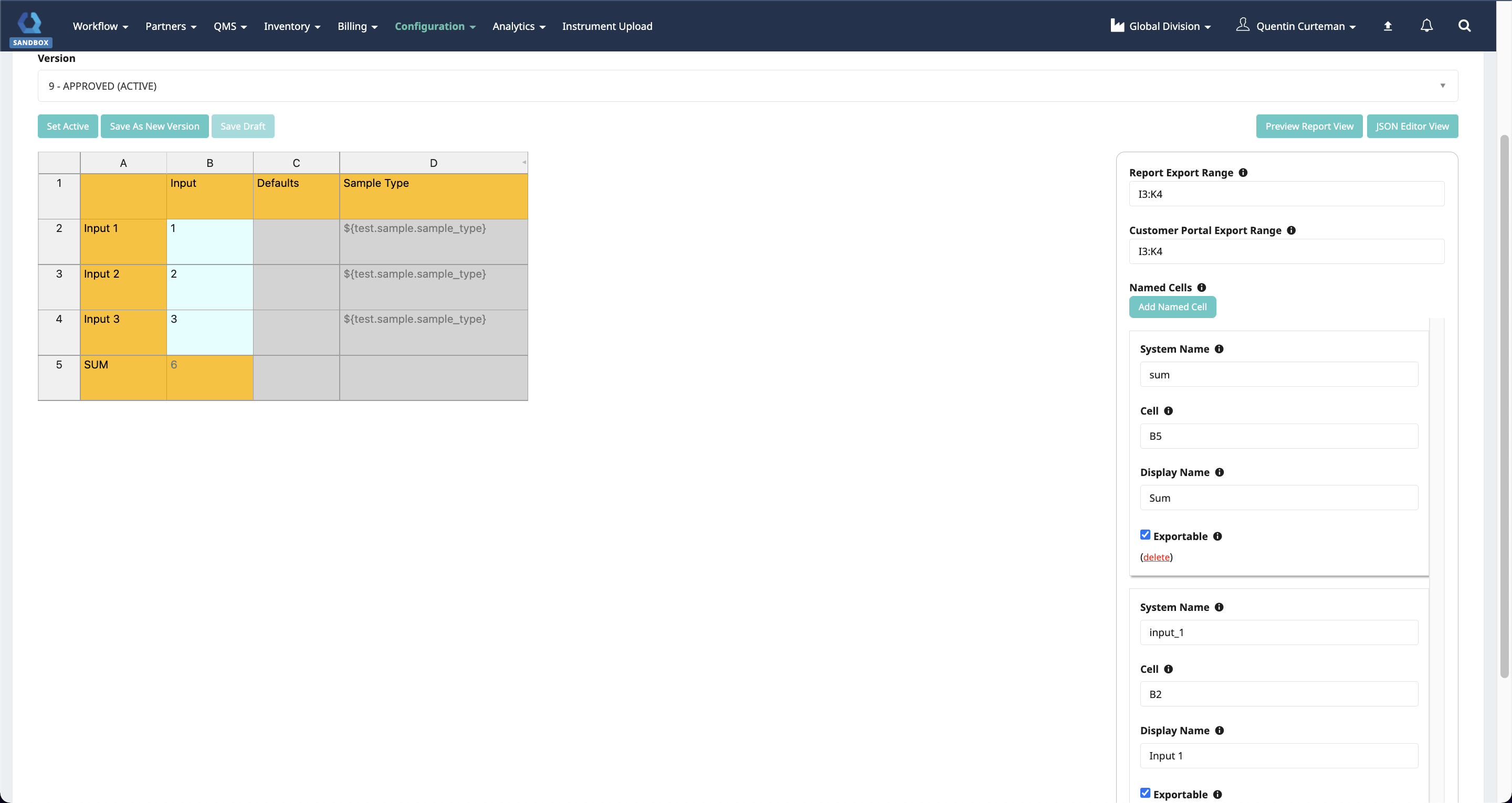
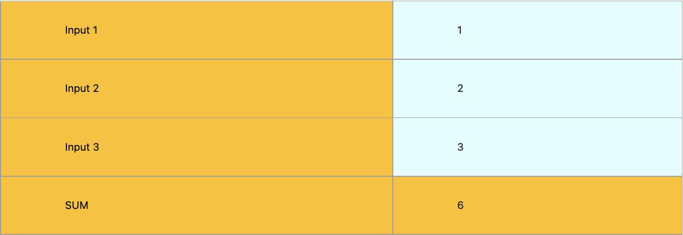
We can define the cell `B5` to be the `sum` field and even give it a display name of `Sum`. Now, we can easily access the value of this cell in reports and in worksheet exports throughout the LIMS.
{{ test.get_worksheet_value("sum") }}

Returns "6"
{{ test.get_worksheet_display_name("sum") }}

Returns "Sum"
Also, observe that we have defined cells A2:B5 to be our export ranges for both Reports and the Customer portal. Below is an example of what this would look like in both the Report and the Customer Portal.
Cell Types
To edit a cell type, highlight a cell or range of cells and right click on the highlighted area. Select "Customize Cell Type" to open the edit modal.
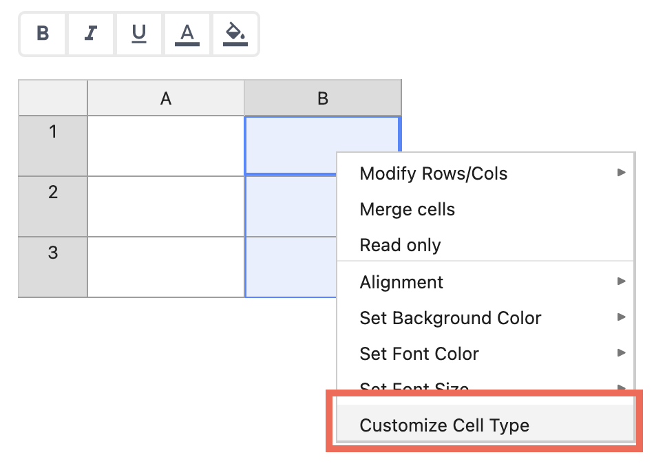
From here, you can change the cell type of the range of cells you have selected.
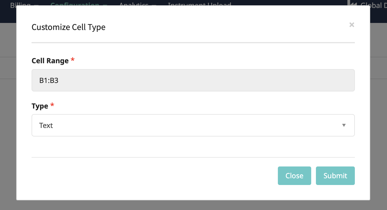
Options
Text
This is the default field type and allows for any input value.
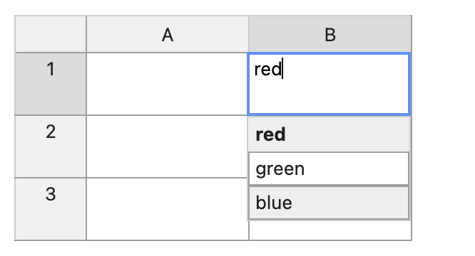
Dropdown
Define a set of options using a valid JSON array to have a cell display in a dropdown format.
Example:
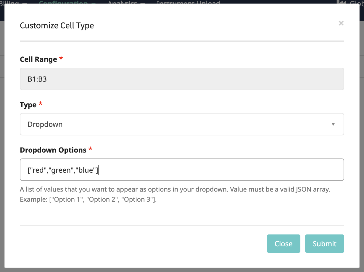
will format the cells as such:
Calculations
Our spreadsheet worksheets are powered by a library called Hyperformula. This library allows for Excel/Google Sheets type actions inside any cell. For example, we can have a cell that represents the sum of other cells using this format:
=SUM(A1:C3)
Simply add this to the value of a cell and the calculations will automatically run whenever the worksheet is updated. Always set cells with a Hyperformula Calculation to be read-only (see Worksheet Config Nuances for more information).
Below are some helpful links to the Hyperformula documentation:
- Referencing a cell's data
- Comparison operators
- Available Logical Functions (and other useful functions!)
- Excel/Google Sheets differences
Dollar References
Summary
Sometimes you may need to reference data from the entity that the worksheet has been assigned to. This can easily be accomplished using a dollar reference inside a cell. Always set cells with a dollar reference to be read-only (see Worksheet Config Nuances for more information).
Reference Examples:
In these examples, we're going to assume we're working in a Spreadsheet Worksheet that has been assigned to a Test. These structures can be applied to whatever datatype the worksheet is assigned to (Batch, Log Entry, etc.).
- ID
-
${test.id}
-
- Relationship
-
${test.sample.sample_type}
-
- Additional Field (Number, Text, Textbox, Checkbox, Dropdown, Hyperlink, Rich Text)
-
${test.additional_fields['text_field_name'].value}
-
- Additional Field (Date)
-
${test.additional_fields['date_field_name'].date_value}
-
- Additional Field (Datetime)
-
${test.additional_fields['datetime_field_name'].datetime_value}
-
- Additional Field (Object Relation)
-
${test.additional_fields['object_relation_field_name'].get_referenced_obj().first_name}
-
You can also add dollar references inline with other strings to dynamically create strings. Example:
${test.id}_value
can print out as
123_value
Working Example
Suppose we have a worksheet defined as such:
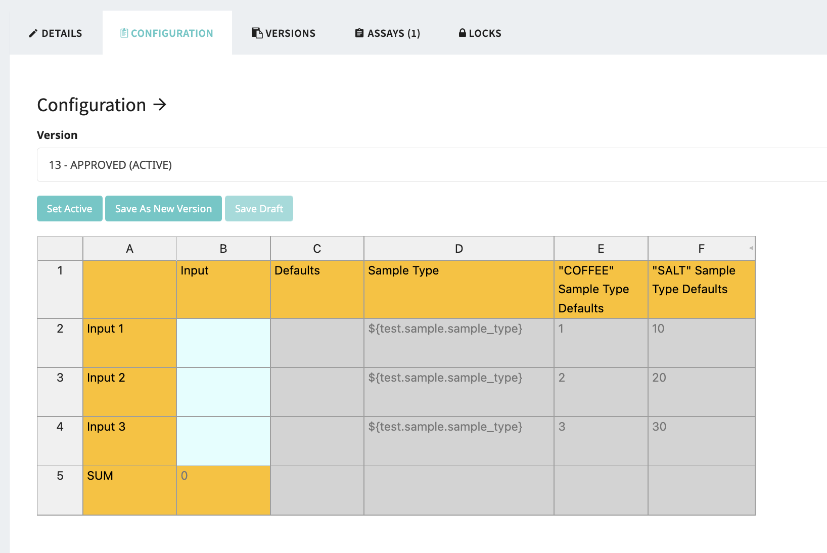
and suppose I have a Sample that has a Sample Type of "COFFEE". When this worksheet is applied to a Test, the worksheet will look like so:
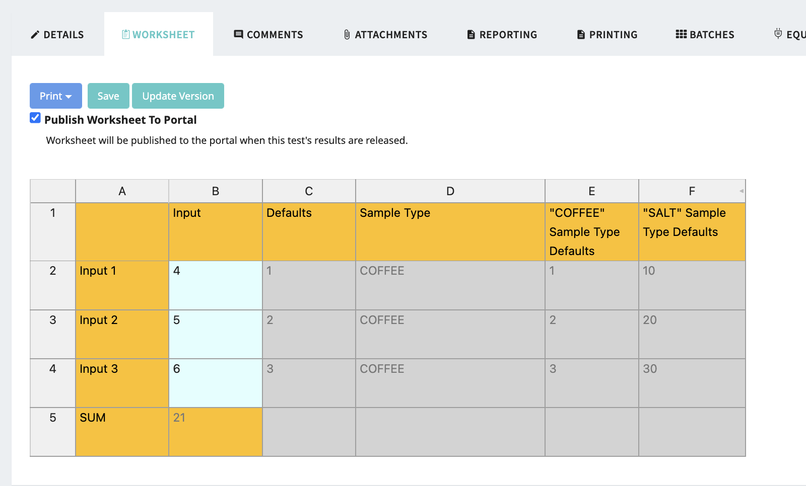
Some things to note from the above example:
- The "Sample Type" column cells of "${test.sample.sample_type}" has been replaced with the actual value saved on the Sample.
- The "Defaults" column has logic in each cell to have a different cell value based on what its corresponding "Sample Type" cell is set to. Here is an example of the cell logic stored in Cell
-
C2=IF(D2="COFFEE", E2, IF(D2="SALT", F2, ""))
-
- The Calculation for the SUM cell has been automatically calculated to include the values input by the Lab user and the Defaults that were populated by the Sample Type.
Continuing with this example, let's suppose that the Sample Type on our Sample is changed to "SALT". The following is what the Test worksheet will show next time the test worksheet page is loaded:
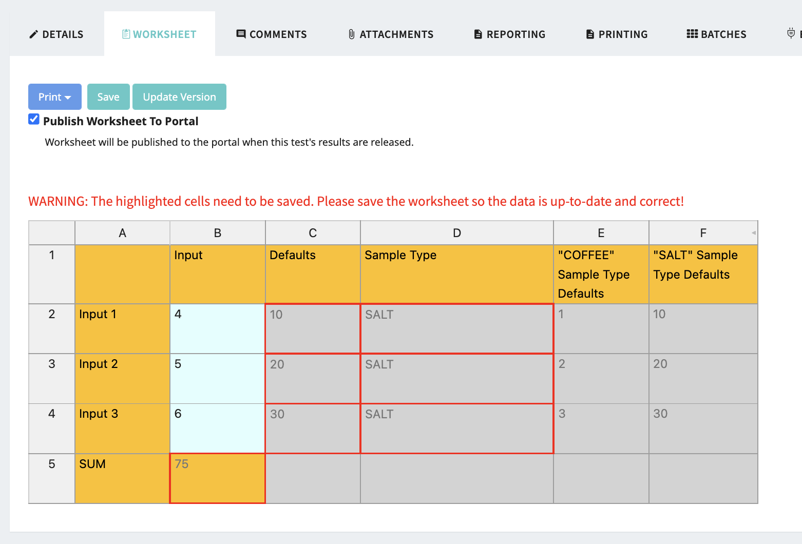
This warning appears when the data in the worksheet that is saved is "stale" and needs to be updated. All you need to do is save the worksheet and this warning will disappear.
Worksheet Config Nuances
Default Values, Calculation Cells, Dollar References and Read-Only Fields
If you have a cell that has a default value in it, is a Hyperfomula Calculation, or is a dollar reference field (Example: "${sample.sample_type}"), you must make the cell read-only. If you do not make the cell read-only, the cell value will not be dynamic. Some issues that this could cause:
- Given I have a worksheet where Cell A2 has a Default Value of "123" and it is not read-only. Assume I create a Test where this worksheet has been applied and I have entered in some data and saved the worksheet. Now suppose I want the Default Value of A2 to be "456". When I save the new worksheet version in the worksheet configuration and update the worksheet version on the Test, the Default Value of Cell A2 will not update to "456".
- Given I have a worksheet where Cell A2 has a Hyperformula calculation in it of "=SUM(A1:B1)". Now assume this worksheet has been applied to a Test and the worksheet has been saved. If either of the values in Cells A1 or B1 change, the calculated value in Cell A2 will not re-calculate.
- Given I have a worksheet where Cell A2 has a value of ${sample.sample_type} and it is not read-only and a Test whose Sample has a "Sample Type" of "COFFEE" Now, assume this worksheet has been applied to the given Test and I have entered in some data and saved the worksheet. Supposed the Lab needs to change the "Sample Type" on the Sample to "SALT". The value in Cell A2 will not dynamically update to "SALT" if the cell has not been defined as read-only.
A good rule of thumb is to make all cells read-only, except the cells that will be directly used to enter data into.
Import/Export
You can import and export spreadsheets in QBench using the buttons highlighted in the image below. 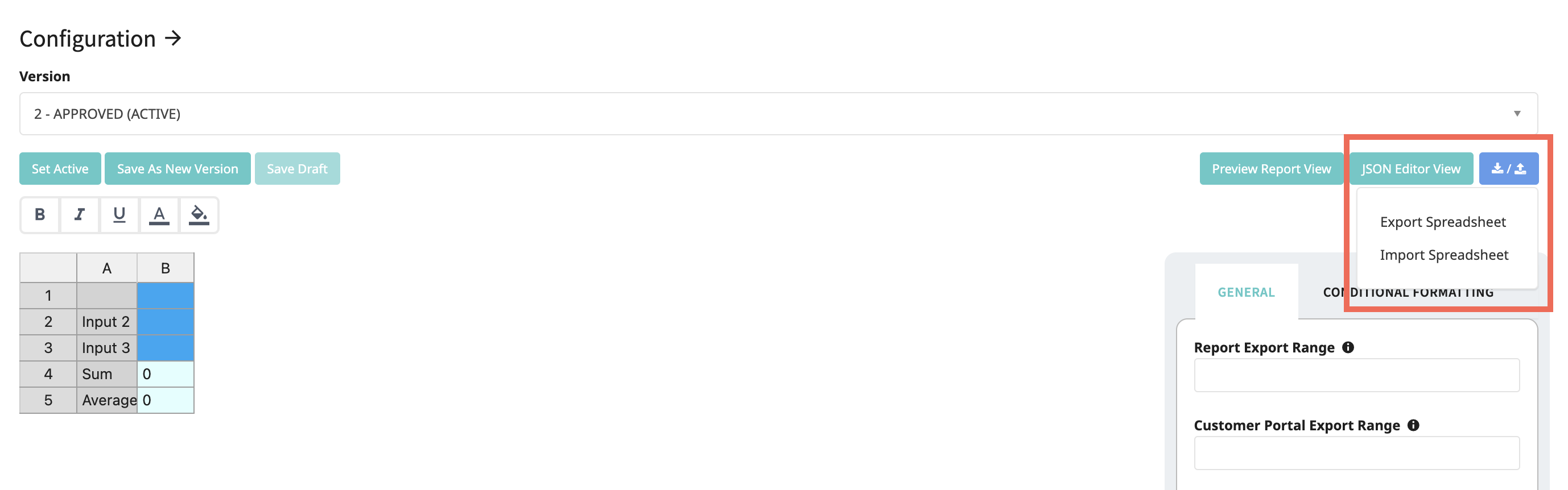
Simply click "Export Spreadsheet" and a JSON file will be downloaded to your local computer. You can then navigate to another spreadsheet worksheet and click "Import Spreadsheet" and select the JSON you have saved to your local computer.
The import and export will contain every aspect of the spreadsheet:
- Cell formatting
- Text
- Readonly cells
- Conditional formatting
- Ranges defined/Named cells
- etc.
A simple use case for this is for transferring a worksheet from a sandbox environment to a production environment.
Conditional Formatting
Summary
Conditional formatting allows for the user to dynamically update a cell or a range of cells formatting and style based on a rule.
Fields
Name
Optional: Add a name to this conditional formatting rule that will appear in the list of conditional formatting rules.
Range
A single cell or range of cells (B4 or B1:C3 for example) where this conditional formatting rule should be applied.
Note: You can add multiple ranges using a comma. Example "A1,B2:B3,C2".
Rule
Rule that will be used to compare the cells value defined in the Range.
Value
Value to compare against the cells value defined in the Range.
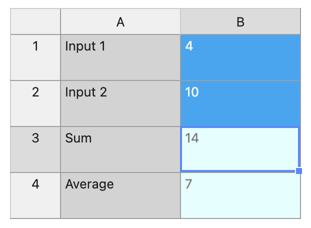
Example
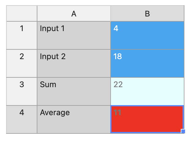
Given this simple Spreadsheet worksheet, suppose we want to make the background color of the "Average" red if its value is greater than 10.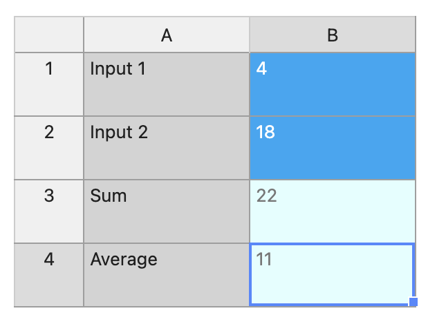
Next:
- Click on the cell you want to apply conditional formatting to. In our case, we select the cell "B4", as it shows in the image above.
- Now click on the "Conditional Formatting" tab on the right hand side and press the "Add Another Rule" button.
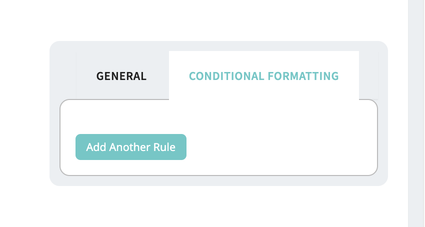
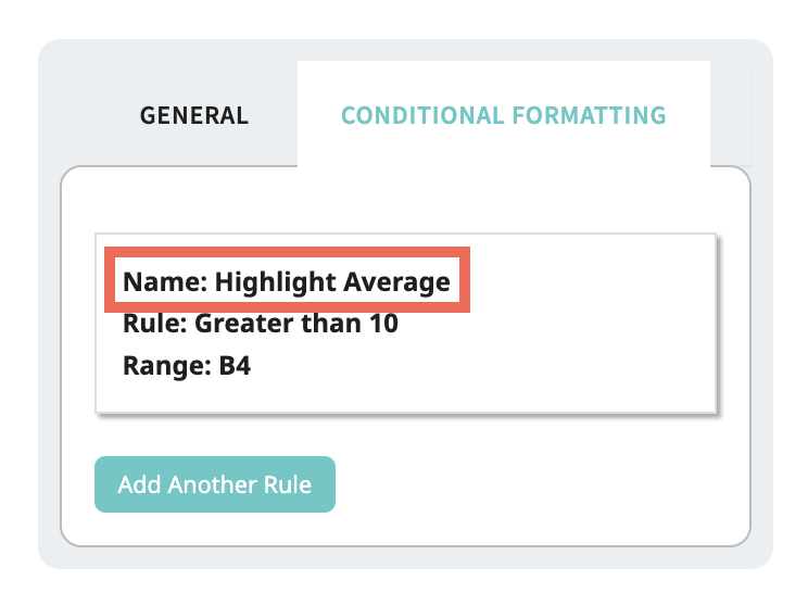
- You should now see a panel of options like so
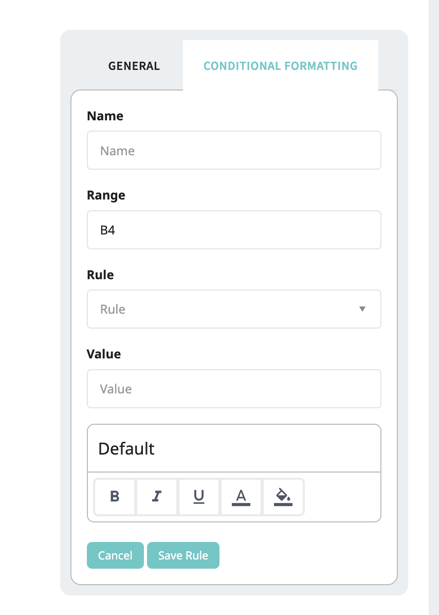
NOTE: Observe how the range is pre-filled with the cell we have selected. If we selected a range of cells, that range would pre-fill as well.
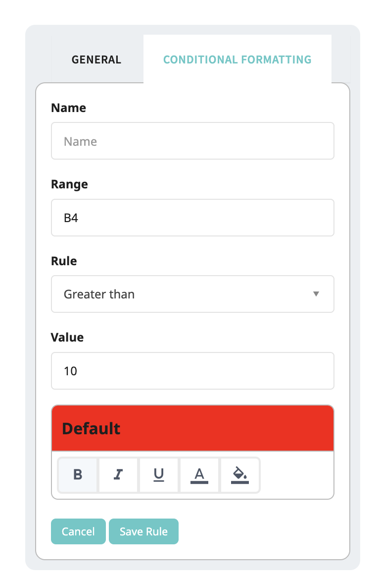
- In the "Rule" field, select the "Greater than" option
- Enter 10 into the "Value" field
- Set the background color to "Red" and make the font "Bold" by clicking on the "Bold" button. It should look like so:
We can now see how the value in the "Average" cell formatting dynamically updates as its value is changed.
Notes
- If you add more rows/columns to your table, you will need to update your conditional formatting range to match its new range if necessary.
- Conditional formatting styles will override any styles that previously existed in a cell if its rule is met.
- To view existing conditional formatting rules, simply highlight over a cell or a range of cells and any conditional formatting rules will appear in conditional formatting tab the toolbar on the right hand side.
Comments
0 comments
Please sign in to leave a comment.